CFOP multi-stage solver
Optimal move counts for all five CFOP stages: Cross / XCross / XXCross / XXXCross / F2L. Lehmer permutation encoding for compact state; a conjugation trick lets four F2L slots share one prune table; cross-stage lower-bound propagation skips iterations below the previous stage's optimum. 1.2M WCA scrambles × 5 stages × 6 orientations = 36M optimal searches — quantifying the marginal value of color neutrality.
Problem statement
A 3×3×3 cube has 8 corners, 12 edges and 6 fixed centres (centre orientations are constant relative to each other). Quotienting by the equivalent whole-cube rotations of the top-centre triple gives
|Cube| = 8! · 38 · 12! · 212 / 12 ≈ 4.3252 × 10¹⁹.The denominator 12 quotients out the orientation of the top centre triple: each physical state corresponds to 12 representations (4 z-axis rotations × 3 vertical orientations) that are identical to the puzzle but differ in labelling.
The CFOP (Fridrich) method splits a solve into four phases: Cross (bottom cross), F2L (First Two Layers), OLL (Orientation of Last Layer — last-layer top colour aligned), PLL (Permutation of Last Layer — last-layer pieces permuted). The first two are the most geometric, have the largest state space, and dominate move count. CubeRoot's std solver decomposes the first block — cross through completed F2L — into five optimal sub-goals:
- Cross: with bottom-face colour D, place and orient the 4 bottom edges so that the down face shows a cross. The 4-edge state is then fixed; we denote that set as X₀. State space |Cross| = 190,080 (see §05).
- XCross: Cross plus one solved F2L pair (1 corner + 1 edge), i.e. first pair finished alongside the cross.
- XXCross / XXXCross: Cross plus 2 / 3 F2L pairs, slot subsets chosen 4-choose-2 / 4-choose-3.
- F2L (XXXXCross): Cross plus all 4 F2L pairs — the entire first two layers solved.
The distance metric is HTM (Half-Turn Metric): U / U' / U2 each count as 1 move. Given a scramble s and goal set G, the solver computes the optimal distance
d(s, G) = min { |alg| : alg(s) ∈ G }Exact optimum for every stage, not an approximation; all 6 orientations for color-neutral analysis; ~5 ns amortized per solve, enabling 2.4M samples × 5 stages × 6 views = 72M optimal searches on a single workstation in under a day.
Four core contributions
- Cast Cross / XCross / F2L optimal-move-count as shortest-path search on a sub state-space, with a compact integer-index encoding.
- Build a precomputation pipeline for move tables and prune tables; pin down 4-bit packed storage and reverse-BFS filling.
- Dissect the multi-slot F2L implementation: conjugation, slot ordering with early exit, paired neighbour/diagonal Huge prune tables, and cross-stage lower-bound propagation.
- Run large-sample statistics on 1,200,000 WCA historical scrambles + 1,271,727 WY-hard scrambles (~2.4M total), quantifying the marginal value of color neutrality and empirically verifying cubic symmetry.
Why brute force fails
Plain BFS branches by 18 moves (6 faces × 3 rotations) at every node. After legal-move filtering (collapse same-face sequences, force a canonical order between opposite faces) the effective branching factor is roughly 13 ~ 15. Optimal Cross is 4 ~ 8 moves, XCross 5 ~ 9, F2L up to 15. Back-of-envelope:
138 ≈ 8.16 × 10⁸, 1312 ≈ 2.33 × 10¹³, 1315 ≈ 5.12 × 10¹⁶.Depth 12 already hits ~2.3 × 10¹³ nodes — at 1 ns per node that's 6+ hours for a single scramble × stage × orientation. Across 2.4M scrambles × 5 stages × 6 views = 72M searches, brute force is hopeless. Two levers bring it back:
- Precompute the state transition per move into move tables — runtime is O(1).
- Precompute the true optimal lower bound from each state to the goal as a prune table. IDA* uses it for cutoffs. The bound is strictly admissible, so the optimum is guaranteed.
Graph-theoretic formulation
Let the move set be
M = { U, U', U2, D, D', D2, R, R', R2, L, L', L2, F, F', F2, B, B', B2 }.Each legal state s ∈ V; there is an edge (s, s') ∈ E iff some m ∈ M satisfies m(s) = s'. The 18 basic moves form 9 inverse pairs (U ↔ U', U2 ↔ U2, etc.): if s can reach s' there is always a return path, so G = (V, E) is an undirected graph with all edge weights = 1. Optimal-Cross-distance equals the shortest path from the scramble s to the goal vertex set G_cross (every Cross-solved state). The canonical move ordering (collapse same-face, enforce an order on opposite faces) drops the branching factor to 12 ~ 15.
The legal-move filter (cube_common.cpp):
// 编号约定: 0:U 1:D 2:L 3:R 4:F 5:B; face = i / 3
// 同面 (i/3 == prev/3) 直接禁掉 — 后一个动作会和前面合并;
// 对面 (axis 相同) 强制 prev 编号大 — 给对面对儿排个序去重。
for (int prev = 0; prev <= 18; ++prev) {
  for (int i = 0; i < 18; ++i) {
    bool bad = (prev < 18) && (
        i/3 == prev/3 ||
        ((i/3)/2 == (prev/3)/2 && (prev/3) % 2 > (i/3) % 2));
    if (!bad) valid_moves_flat[prev][cnt++] = i;
  }
}
The result: valid_moves_count[prev] sits at 12 ~ 15, a 17 ~ 33% expansion saving over plain 18. At IDA* depth 12 ~ 15 that compounds to 1 ~ 2 orders of magnitude overall. prev = 18 is the "no predecessor" sentinel, giving the root all 18 choices.
Five analyzer variants
One shared move-table + prune-table backbone, five variants by re-defining the goal:
| Variant | Executable | Cross goal | Notes |
|---|---|---|---|
std | std_analyzer.exe | Standard Cross | Primary focus (no extra constraint); optimal over all 5 stages |
pseudo | pseudo_analyzer.exe | Pseudo Cross | D layer may sit at any 90/180/270° offset; looser goal |
pair | pair_analyzer.exe | Cross + 1 Pair | Cross plus one F2L pair finished together; stricter goal |
pseudo_pair | pseudo_pair_analyzer.exe | Pseudo Cross + Pair | Both relaxations combined |
eo_cross | eo_cross_analyzer.exe | EO + Cross | Cross plus full Edge Orientation on all 12 edges |
This page focuses on std: its goal is closest to the real-competition Cross / XCross definitions and serves as the baseline for the other variants. The others appear only in the comparison table below.
Mean move counts on WCA 1.2M, all five variants, Cross / XCross stages (BGORWY full color-neutral):
| Variant | Cross mean | Cross median | XCross mean | XCross median | Δ vs std/Cross |
|---|---|---|---|---|---|
| std | 4.811 | 5 | 6.536 | 7 | 0 |
| pseudo | 4.308 | 4 | 5.530 | 6 | −0.503 |
| pseudo_pair | 4.506 | 5 | 5.806 | 6 | −0.305 |
| pair | 5.371 | 5 | 7.124 | 7 | +0.560 |
| eo_cross | 6.427 | 7 | 7.813 | 8 | +1.616 |
Where the variants come up, and how they relate to std:
- pseudo accepts any 90/180/270° offset on the D layer as solved; ~0.5 moves shorter than std. Used as a setup stage in some advanced methods that allow a D-layer offset, e.g. EOCross+1 and roux-blindfold variants.
- pair requires one F2L pair simultaneously with the Cross — equivalent to a fixed-slot version of std's XCross sub-goal. The three-way inequality is strict:
std/Cross < pair/Cross < std/XCross(4.811 < 5.371 < 6.536). - eo_cross additionally requires all 12 edges fully oriented on top of Cross — the strictest goal; ~1.6 moves longer than std on average. This is the canonical first-block of the ZZ method, the speedsolving system proposed by Zbigniew Zborowski.
- The other 4 variants share the std algorithmic skeleton verbatim — they differ only in prune-table goal states, sub-state dimensions, and a few EO-specific move tables (e.g. mt_eo12). The Lehmer / move-table / prune-table / IDA* / conjugation / cross-stage-propagation scaffolding works unchanged for all four.
Sub state-space sizes
The Cross sub-problem tracks 4 bottom edges (in canonical orientation: E8, E9, E10, E11). Each edge has 12 positions × 2 flips = 24 slot/orientation pairs, distinct between the four edges, so
|Cross| = 24 · 22 · 20 · 18 = 190,080.XCross adds one F2L pair (1 corner + 1 edge) on top of Cross, each with 24 states:
|XCross| = 190,080 · 24 · 24 = 109,486,080 ≈ 1.09 × 10⁸.XXCross adds 2 F2L pairs:
|XXCross| = 190,080 · 242 · 242 ≈ 6.30 × 10¹⁰.By XXXCross / F2L the full product space is too large to materialise as one table. Hence the "Huge neighbour / diagonal prune tables" + a conjugation trick (§10, §12) that lets four slots share a single precomputation.
Lehmer permutation encoding
Single-edge / single-corner state values
Each edge cubie's state combines its current slot index p with its orientation o:
v_edge = 2p + o, p ∈ {0, ..., 11}, o ∈ {0, 1}.That gives 12 × 2 = 24 states per edge, the constant StateSpace::EDGE = 24 in code. Corners likewise:
v_corn = 3p + o, p ∈ {0, ..., 7}, o ∈ {0, 1, 2}.Also 8 × 3 = 24 states (StateSpace::CORNER = 24). Every per-cubie index used by Cross / XCross / F2L sits on these two 24s.
Combining cubies: the Lehmer code
Sparse indexing wastes memory: naive 244 = 331,776 cells for 4 edges, while only 190,080 are legal (~57% utilization). Lehmer code (factorial number system) maps "ordered choice of k from n" onto [0, P(n,k)) compactly. For Cross:
|Cross| = P(12, 4) · 24 = 11,880 · 16 = 190,080.The rule: list all length-n ordered choices in lexicographic order; the Lehmer code is the row number. A minimal example — pick 2 of {0, 1, 2}, P(3, 2) = 6 permutations sorted lexicographically:
(0,1) → 0, (0,2) → 1, (1,0) → 2, (1,2) → 3, (2,0) → 4, (2,1) → 5.Encoding is closed-form, not a table lookup. For each position i: count t_i = "elements to the left of a_i that are smaller". The rank of a_i in "remaining choices" is a_i − t_i; multiply by the factorial weight for the remaining positions and sum. Example for (1, 2): a₀ = 1 has rank 1, weight P(2, 1) = 2 → 1×2 = 2. a₁ = 2 (1 used on the left, rank = 2 − 1 = 1), weight P(1, 0) = 1 → 1. Total 3 — matches the table above.
General form (k-of-n ordered choice):
index = Σᵢ (aᵢ − tᵢ) · P(n − 1 − i, k − 1 − i).The implementation factors out an orientation slice (c = 2 or 3) as a c-ary integer, divides the raw array by c to get a pure permutation, applies the Lehmer formula above to that, then linearly combines them. Three parameters:
c= orientation base (edges c = 2, corners c = 3)pn= total cubies of this type (edges 12, corners 8)n= cubies actually encoded (Cross uses 4 edges, XCross adds 1 corner + 1 edge)
base_array and c_array are factorial-base weight tables, initialised at startup. They hold "remaining-position permutation weight" and "remaining-position orientation c-ary weight" respectively.
int array_to_index(const vector<int>& a, int n, int c, int pn) {
  int idx_p = 0, idx_o = 0, tmp;
  // (1) orientation: low c-ary digits
  for (int i = 0; i < n; ++i)
    idx_o += (a[i] % c) * c_array[c][n - i - 1];
  // (2) position: Lehmer code over a[i] / c
  vector<int> pa = a;
  for (int i = 0; i < n; ++i) pa[i] /= c;
  for (int i = 0; i < n; ++i) {
    tmp = 0;
    for (int j = 0; j < i; ++j)
      if (pa[j] < pa[i]) tmp++;
    idx_p += (pa[i] - tmp) * base_array[24 / pn][i];
  }
  return idx_p * c_array[c][n] + idx_o;
}
Decoding inverts: pull out the c-ary orientation digits, then walk a shrinking "remaining values" list driven by the Lehmer coefficients. The map is a bijection, so every prune-table cell corresponds to exactly one real state — no holes, no collisions.
Cross split into two half-groups
Encoding the 4 cross-edges as a single 190,080-index gives a ~93 KB prune table; but the Cartesian product with Corner / Edge dimensions plus mt_edge4's 24-stride bloats it fast at higher stages. The Cross solver picks a lighter alternative: split the 4 edges into two disjoint half-groups {E8, E9} and {E10, E11} and index each by its own EDGE2:
|S_Edge2| = 24 · 22 = 528, 528 · 528 = 278,784 ≈ 140 KB.constexpr int EDGE2 = 528; // 单半组的状态空间大小
constexpr int EDGE2_A_SOLVED = 416; // {E8, E9} 的 Lehmer 秩 × 2² = 104×4
constexpr int EDGE2_B_SOLVED = 520; // {E10, E11} 的 Lehmer 秩 × 2² = 130×4
constexpr int CROSS_SOLVED = 187520; // 整 Cross 已解状态的整体索引The Cross prune table pt_cross addresses by the pair (i₁, i₂):
idx_cross = i₁ · EDGE2 + i₂, i₁, i₂ ∈ [0, 528).The split is lossless: the two halves occupy disjoint slot sets ({E8, E9} vs {E10, E11}) so they never collide; you can encode them independently without losing any information, while drastically reducing storage when combined with Corner / Edge dimensions later.
Move tables
A physical-geometry transition costs O(n) per node (n = tracked cubies); at IDA* depth 12 that compounds to ~10¹³ — unacceptable. Tabulate "(state index, move) → next state index" once: O(|S| · |M|) memory in exchange for O(1) transitions.
mt[s · |M| + m] = T(s, m).In the IDA* inner loop, the typical access pattern is "read the table, descend immediately": next time, s is the returned value. Doing s × |M| each time means a multiplication by 18, which isn't a power of two and can't be shift-optimised. createMultiMoveTable stores the "pre-multiplied by |M|" offset instead, so chained lookups need only addition:
s_next = mt[s_cur + m].s stays in the "already × |M|" form. Source createMultiMoveTable writes mt[18·tmp + inv[j]] = i (the backward-fill path) which respects this convention; each state owns 18 contiguous slots.
mt_edge4: a non-18 stride
The hottest path (XCross search_1) needs three lookups per node: the 4-edge Cross table mt_edge4 + 1 corner mt_corn + 1 edge mt_edge. If all three used 18 stride, index synthesis would need extra multiplications. The source gives mt_edge4 a 24 stride (built by createMultiMoveTable2 rather than createMultiMoveTable): each cell stores next_index × 24.
24 is chosen because 24 = single-corner state count = single-edge state count (see §06: EDGE = CORNER = 24). In search_1 the next Cross-state n_i1 is therefore already × 24; we just add the [0, 24) corner index to get "Cross_idx × 24 + corner_idx", then × 24 + edge index → 3-D joint index. One multiplication for the whole step. The cost is mt_edge4 using (24 − 18)/18 ≈ 33% more memory than the 18-stride form (~4.3 MB) — acceptable.
| Table | Tracks | |S| | Stride | Entries |
|---|---|---|---|---|
| mt_edge | single edge | 24 | 18 | 432 |
| mt_corn | single corner | 24 | 18 | 432 |
| mt_edge2 | 2-edge group (Cross half) | 528 | 18 | 9,504 |
| mt_edge3 | 3-edge group | 10,560 | 18 | 190,080 |
| mt_corn2 | 2-corner group | 504 | 18 | 9,072 |
| mt_corn3 | 3-corner group | 9,072 | 18 | 163,296 |
| mt_edge4 (× 24) | 4-edge group (full Cross) | 190,080 | 24 | 4,561,920 |
| mt_edge6 | 6-edge group (paired with Huge) | 42,577,920 | 18 | 766,402,560 |
mt_edge6 alone is ~3 GB; runtime maps it read-only via mmap, avoiding a single big alloc while still benefiting from the OS page cache. The other 7 tables stay resident in RAM. All .bin files are produced once offline by table_generator.exe into the tables/ directory; the solver just loads them at startup, no runtime computation.
Prune tables
For each (indexed) sub-state s store the true shortest distance to the goal set, h(s). During an IDA* iteration with bound D, if g moves have been made and g + h(s) ≥ D, the branch cannot reach the goal within D moves — prune and backtrack. The required property is admissibility:
∀ s: h(s) ≤ d(s, goal).If h never overestimates (admissible), IDA*'s first solution is globally optimal. If admissibility fails, only an approximation is guaranteed. That's why every prune table here uses a reverse-BFS-computed exact distance within its sub-state space: that distance is genuinely shortest in the projection, so it strictly bounds the real distance from above.
Reverse-BFS fill (source: prune_create.cpp::createPTCrossCE): seed goal cells with 0; each round expand all 18 inverse moves of cells already at depth d and set unmarked neighbours to d+1, until the table is full. Parallel writes use OpenMP + CAS to avoid locks; early termination when a round adds 0 new cells:
tmp[start_idx] = 0;
for (int d = 0; d < depth; ++d) {
  int nd = d + 1;
  #pragma omp parallel for reduction(+ : cnt)
  for (long long i = 0; i < total; ++i) {
    if (tmp[i] != d) continue;
    // expand 18 neighbours of i
    for (int j = 0; j < 18; ++j) {
      long long ni = move_table_lookup(i, j);
      unsigned char expected = 255;
      __sync_val_compare_and_swap(&tmp[ni], expected, nd);
    }
  }
}
Per-stage diameters under std are ≤ 12 (15 only for F2L on single-W); 4 bits (0 ~ 15) suffice, two cells per byte halves storage — critical for tables ranging from tens of MB to 10 GB. The macros in prune_tables.h:
inline int get_prune(const unsigned char* table, long long index) {
  return (table[index >> 1] >> ((index & 1) << 2)) & 0xF;
}

inline void set_prune(vector<unsigned char>& table, long long index, int value) {
  int shift = (index & 1) << 2;
  table[index >> 1] &= ~(0xF << shift);
  table[index >> 1] |= (value & 0xF) << shift;
}
index >> 1 is the byte address; (index & 1) << 2 is a shift of 0 or 4, deciding low or high nibble; & 0xF masks out the 4-bit value.
| Prune table | Sub-state | Index space | Storage (4-bit) | Load mode |
|---|---|---|---|---|
| pt_cross | Cross 4 edges | 278,784 | ~ 140 KB | resident |
| pt_cross_C4E0 | Cross + 1 corner + 1 edge (XCross) | 1.09 × 10⁸ | ~ 52 MB | resident |
| pt_cross_C4C5E0E1 (Huge NB) | Cross + 2 neighbour pairs | ~ 2.14 × 10¹⁰ | ~ 10 GB | mmap on demand |
| pt_cross_C4C6E0E2 (Huge DG) | Cross + 2 diagonal pairs | ~ 2.14 × 10¹⁰ | ~ 10 GB | mmap on demand |
Admissibility & the optimality theorem
Because each prune table stores the exact shortest distance within its sub-state space (call it h*), we use h(s) = h*(s_sub) where s_sub is the projection of the full cube state s onto the sub-state. Shortest paths in the full space can only be at least as long as in the projection (the full space has more constraints — the projection ignores some cubies), so:
h(s) = h*(s_sub) ≤ d(s, G).So h is non-overestimating — admissibility holds strictly. Combined with IDA*'s iterative deepening (DFS bounded by an integer D that grows by 1 per round starting from the initial lower bound), the proof is short: the first solution found, at some depth D, equals the optimal move count. This is the mathematical bedrock under all of the solver's numeric claims.
IDA* search loop
IDA* (Iterative Deepening A*) was introduced by Korf in 1985 to solve A*'s memory blow-up on large state spaces. The core idea combines DFS's linear memory with A*'s heuristic pruning:
- Each round sets a depth bound D and runs a DFS with heuristic pruning;
- If no solution at D, set D ← D + 1 and retry;
- Search is a single-path DFS, so space is just O(D).
For each node s, look up h(s) first; if g + h(s) ≥ D, prune. Restarting from the root each round looks wasteful, but because the search tree grows exponentially with depth, the deepest round alone usually accounts for 95%+ of total runtime — redo cost is amortised away.
Pseudocode
function IDA_STAR(s_root):
  D ← h(s_root)                     // 初始深度上限
  while True:
    found, new_D ← DFS(s_root, 0, D)
    if found: return D              // 找到解, 即为最优
    if new_D = ∞: return None       // 不可达
    D ← new_D

function DFS(s, g, D):
  if g = D and s ∈ goal: return (True, _)
  f ← g + h(s)
  if f > D: return (False, f)       // 超出深度, 记录下次的最小 f
  next_D ← ∞
  for m in valid_moves[prev]:
    s' ← move_table[s, m]
    found, t ← DFS(s', g + 1, D)
    if found:    return (True, _)
    next_D ← min(next_D, t)
  return (False, next_D)
The source code does not bother to track next_D; it just runs for (D = h(s_root); D ≤ MAX; D++), since every stage has a known diameter (Cross ≤ 8, XCross ≤ 12, F2L ≤ 15). This trade gives up a small win ("skip the exact next-D") for extreme implementation simplicity. The first hit is optimal because the heuristic is admissible.
Cross solver: cross_solver.h
Wiring move tables + prune tables + IDA* into 71 lines of C++ gives CrossSolver, the cleanest component in std_analyzer:
struct CrossSolver {
  const int *p_mt_edge2;
  const unsigned char *p_pt;          // Cross 剪枝表

  CrossSolver() {
    p_mt_edge2 = MoveTableManager::getInstance().getMTEdge2Ptr();
    p_pt       = PruneTableManager::getInstance().getCrossPTPtr();
  }

  bool search(int i1, int i2, int depth, int prev) {
    const int *moves = valid_moves_flat[prev];
    const int  count = valid_moves_count[prev];
    for (int k = 0; k < count; ++k) {
      int m    = moves[k];
      int n_i1 = p_mt_edge2[i1 + m];                              // (a)
      int n_i2 = p_mt_edge2[i2 + m];                              // (a)
      long long idx = (long long)n_i1 * StateSpace::EDGE2 + n_i2; // (b)
      if (get_prune(p_pt, idx) >= depth)  continue;               // (c)
      if (depth == 1)                     return true;            // (d)
      if (search(n_i1 * 18, n_i2 * 18, depth - 1, m))             // (e)
        return true;
    }
    return false;
  }
};- (a) Two table lookups:i₁ and i₂ are stored pre-multiplied by 18; just add m to step to the next offset — no multiplication.
- (b) Index synthesis:idx = n_i₁ × 528 + n_i₂ — the 1-D offset into the prune table. Because n_i₁ is the true index (already divided by 18), one multiplication is unavoidable here.
- (c) Heuristic prune:If h(s') ≥ depth the branch can't finish in the remaining budget — skip.
- (d) Early accept:When depth = 1 and h = 0 (already filtered out by (c)), the current move lands exactly at the Cross-solved state — return success.
- (e) Recurse:Re-multiply state offsets by 18 (back to the "pre-strided" form), depth − 1, prev ← m, recurse.
Inverse encoding: how get_stats turns a scramble into initial indices
Before calling search, the scramble must be mapped to (i₁, i₂). The obvious route is to simulate the physical state and then encode it; std_analyzer instead uses a tighter inverse trick: start from the solved Cross state (i₁, i₂) = (EDGE2_A_SOLVED, EDGE2_B_SOLVED) and apply each scramble move through the move table. This equals "scramble first, then encode" because move tables are bijections inside the state space.
vector<int> get_stats(const vector<int>& base_alg,
                      const vector<string>& rots) {
  vector<int> res(rots.size(), 0);
  for (size_t i = 0; i < rots.size(); ++i) {
    auto alg = alg_rotation(base_alg, rots[i]);
    int i1 = StateSpace::EDGE2_A_SOLVED;     // 416
    int i2 = StateSpace::EDGE2_B_SOLVED;     // 520
    for (int m : alg) {                       // 逐步施加打乱
      i1 = p_mt_edge2[i1 * 18 + m];
      i2 = p_mt_edge2[i2 * 18 + m];
    }
    long long idx = (long long)i1 * StateSpace::EDGE2 + i2;
    int d_min = get_prune(p_pt, idx);         // 启发式下界
    if (d_min == 0) continue;                 // Cross 已完成
    for (int d = d_min; d <= 8; ++d) {        // IDA* 迭代加深
      if (search(i1 * 18, i2 * 18, d, 18)) {  // prev=18 表示无上一步
        res[i] = d;
        break;
      }
    }
  }
  return res;
}
The payoff: no "physical state → index" conversion code is needed anywhere; the whole analyzer runs on the "initial state + scramble sequence" abstraction. The rots parameter feeds the 6 color-neutrality views (see §15).
search_1: three-dimensional XCross search
Stepping up to XCross adds 1 corner + 1 edge of one F2L slot to track. The function is search_1; slot index is s1. Three key tricks: (a) conjugation, (b) mt_edge4's 24-stride, (c) three-table index synthesis.
bool search_1(int i1, int i2, int i3, int s1, int depth, int prev) {
  const int *moves = valid_moves_flat[prev];
  const int  count = valid_moves_count[prev];
  for (int k = 0; k < count; ++k) {
    int m  = moves[k];
    int m1 = conj_moves_flat[m][s1];                 // (a) 共轭
    int n_i1 = p_mt_edge4[i1 + m1];                  // (b) Edge4: 24-步幅
    int n_i2 = p_mt_corn [i2 + m1];                  //     Corner: 18-步幅
    int n_i3 = p_mt_edge [i3 + m1];                  //     Edge:   18-步幅
    long long idx = (long long)(n_i1 + n_i2) * 24 + n_i3;  // (c)
    if (get_prune(p_pt_cross_C4E0, idx) >= depth) continue;
    if (depth == 1) return true;
    if (search_1(n_i1, n_i2 * 18, n_i3 * 18, s1, depth - 1, m))
      return true;
  }
  return false;
}- (a) Conjugation:m₁ = conj_moves_flat[m][s₁] maps move m into the s₁-slot's frame, so all 4 F2L slots share one prune table. See §10.
- (b) Three table lookups:mt_edge4 has the 24-stride form: its return value is already "next Cross state × 24". mt_corn and mt_edge use the standard 18-stride and return raw indices.
- (c) Index synthesis:n_i₁ already carries the ×24 factor; adding n_i₂ (corner 0..23) builds "Cross_idx × 24 + corner_idx", then × 24 + n_i₃ (edge 0..23) gives the 3-D index — one multiplication total.
Conjugation for slot symmetry
F2L has 4 slots: BL / BR / FR / FL. A separate prune table per slot would need 4 × 10 GB = 40 GB for Huge. Use a y-axis 90° rotation to map every slot back to the same "reference slot" (slot 0):
m' = conj_moves_flat[m][k], k ∈ {0, 1, 2, 3}.To solve in slot k, the scramble and table stay put; the move m we'd execute is rewritten through conjugation m'. The mapping is concrete:
y: F→L→B→R→F (side faces cycle 90°)y2: F↔B, L↔Ry': F→R→B→L→F (reverse)- U / D face moves stay put
The whole conj_moves_flat is an 18 × 4 precomputed table; cube_common.cpp::init_matrix builds it once by enumerating 18 moves × y / y² / y' rules. One indexing at runtime. Geometrically: U → U, D → D (top/bottom moves are fixed) while R / L / F / B rotate R → F → L → B → R per 90° y-rotation, preserving the 90° / 180° / -90° suffix (e.g. R2 → F2, never F). This is the single most important symmetry exploit in the std solver — it collapses 4 × Huge into 1 × Huge.
Slot ordering + early exit
XCross is min over 4 slots: we only want min_k d(s, slot_k). First pull the O(1) prune-table bound h_k per slot, sort the 4 candidates by h_k ascending, then run IDA* in that order:
sort(tasks, [](auto& a, auto& b){ return a.h < b.h; });
int current_best = 99;
for (auto& t : tasks) {
  if (t.h >= current_best) break;          // (1) 下界已超过现存最优,跳过
  int max_search = min(12, current_best - 1);
  int res = 99;
  if (t.h > 0) {
    for (int d = t.h; d <= max_search; ++d) {
      if (search_1(...)) { res = d; break; }
    }
  } else res = 0;
  if (res < current_best) current_best = res;
}
xc_min[r] = current_best;
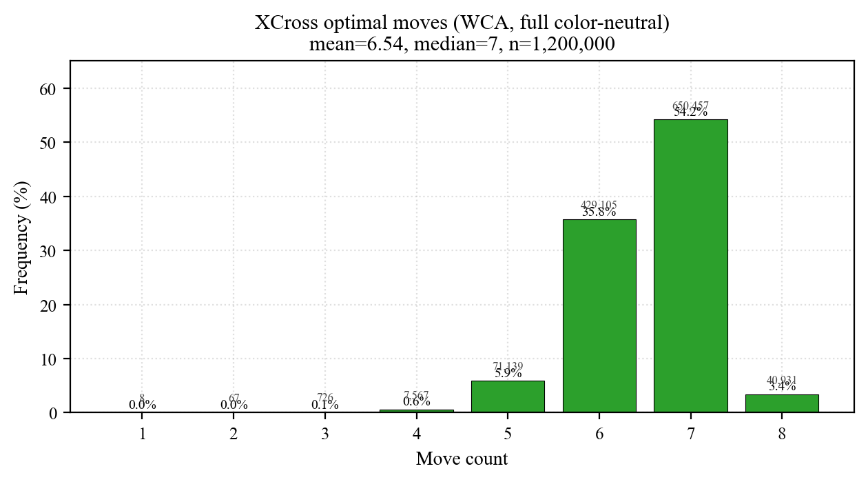
Line (1) is the early exit: once a 7-move XCross is found in one slot, slots with a bound ≥ 7 are skipped entirely. WCA XCross has mean 6.54, std 0.69, mode 7 at 54.20% (BGORWY view). About 50% of scrambles already hit a ≤ 7 answer in the first slot, capping the remaining 3 slots' IDA* depth at 6 via min(12, current_best - 1) — large fractions of the search tree are pruned. Most scrambles only touch 1 ~ 2 slots in practice.
Huge neighbour / diagonal tables
XXCross picks 2 of 4 slots = 6 unordered pairs. F2L's 4 slots = 4-choose-2 = 6 pairs; XXXCross has 4 cases. To share precomputation across "any pair," classify pairs by relative geometry:
- Neighbour (NB): adjacent slots (slot difference ±1 mod 4). e.g. BL+BR, FR+FL — 4 pairs.
- Diagonal (DG): opposite slots (slot difference 2 mod 4). e.g. BL+FR, BR+FL — 2 pairs.
One Huge prune table per class: NB → pt_cross_C4C5E0E1 (Cross + 2 neighbour pairs), DG → pt_cross_C4C6E0E2 (Cross + 2 diagonal pairs). Combined with conjugation, every pair maps to a canonical geometry. Sizes:
|Huge| = |EDGE6| · |CORNER2| = 42,577,920 · 504 ≈ 2.14 × 1010.4-bit packed + mmap, each ~10 GB. For each (scramble, slot pair), the corresponding Huge table first supplies a tight initial lower bound, then every node expansion inside search_2 re-queries that Huge table; if the lookup ≥ remaining depth, the branch is pruned. Because Huge models "full Cross + 2 F2L slot-blocks" jointly, the bound it gives is tighter than the sum of independent per-slot pt_cross_C4E0 queries, allowing cutoffs at shallower depths. search_2 reads Huge directly at XXCross; XXXCross / F2L can also reuse it as a weaker bound. If memory is tight, falling back to pt_cross_C4E0 alone still works — at the cost of a weaker prune and deeper search.
search_3 and search_4: scaling to 3 and 4 slots
search_2 already models the full Cross + two F2L slot-blocks jointly. As slot count grows, the geometric combinations grow too — but every pair of slots is still either neighbour (NB) or diagonal (DG). The Huge tables themselves don't change; only the enumeration of slot-pairs does.
search_3(XXXCross, 3 slots): maintains the standard pt_cross_C4E0 prune across 3 perspectives + 3 Huge-table queries (C(3,2) = 3 slot pairs). Each pair's NB / DG class selects which Huge to query.search_4(F2L, 4 slots): maintains 4 neighbour Huge + 2 diagonal Huge = 6 slot-pair lookups (C(4,2) = 6), covering every geometric relation across the 4 slots. Each search node performs 4 base-prune + 6 Huge ≈ 14 table queries.
From search_2 to search_4 the per-node table query count rises linearly from 4 to 14; but each extra tight lower bound monotonically raises the effective prune rate, so total node count grows slowly, not exponentially, across stages. This is the "many-precise-heuristic-queries for aggressive pruning" trade — under OpenMP on 8 cores, std_analyzer finishes one scramble's 5 stages × 6 orientations = 30 full optimal searches in a few seconds.
Cross-stage lower-bound propagation
Key observation: Cross is a sub-goal of XCross, XCross is a sub-goal of XXCross, so
d(Cross) ≤ d(XCross) ≤ d(XXCross) ≤ d(XXXCross) ≤ d(F2L).The source get_stats solves stages in order and stashes each stage's per-view optimum into xc_min[r] / xxc_min[r] / xxxc_min[r] for the next stage to read. At XXCross, the XCross optimum is known; start IDA* at max(h_prune, xc_min[r]) instead of h_prune, skipping every iteration shorter than the previous stage. If XCross = 7, XXCross starts at 7 — skipping all of 0 ~ 6. Worst case (XCross = 3 and XXCross = 14) skips 11 rounds. WCA distributions show stage-to-stage spread is usually ≤ 2, so IDA* nails 95% of samples in 1 ~ 3 rounds:
// XXCross 起搜深度: 不低于前一阶段最优,也不低于自己的剪枝下界
int startD = std::max(h_prune, xc_min[r]);
for (int d = startD; d <= 14; ++d) {
  if (search_2(..., d, ...)) { res = d; break; }
}
Net effect: each stage starts IDA* close to its terminal depth, collapsing the classical ~D iterations down to ~2. Even though the deepest round of an IDA* re-search typically owns 95%+ of total cost (the search tree is exponential), cross-stage propagation still buys roughly 30% ~ 40% extra speedup on mid-difficulty scrambles — by raising the floor under which the deepest round itself starts. This is why the std solver stays fast even at F2L depth 14 ~ 15.
Large-sample experiments
Two datasets:
- Set 1 (WCA): 1,200,000 official 3×3 scrambles aggregated from 6 events (3×3, OH, BLD, MultiBLD, FMC, Feet). Real competition distribution.
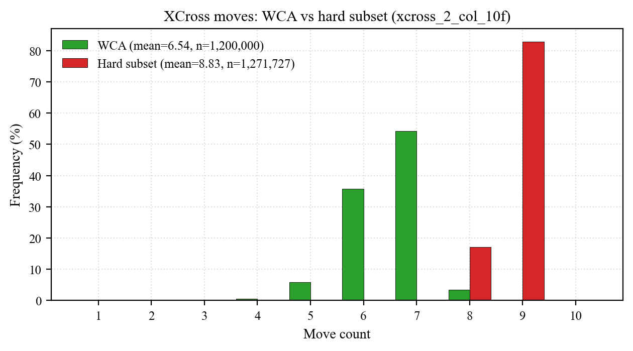
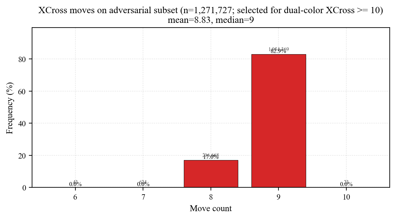
- Set 2 (hard subset): 1,271,727 scrambles whose WY-axis dual-color XCross is exactly 10 moves (single-W and single-Y both need 10). Worst-case stress test for U/D-axis solvers.
Each scramble runs 5 stages × 6 orientations = 30 optimal solves. Total: (1.20M + 1.27M) × 5 × 6 ≈ 74M optimal searches. Output is CSV with 1 (scramble id) + 5 (stages) × 6 (orientations) = 31 columns per row; downstream aggregation takes min over color subsets to derive 14 CN configurations (6 single + 3 dual + 3 quad + 1 hex + 1 baseline).
WCA std five-stage summary
| Stage | Subset | min | max | mean | std | p10 | p50 | p90 | p99 | mode (%) |
|---|---|---|---|---|---|---|---|---|---|---|
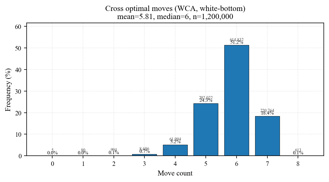
| Cross | W | 0 | 8 | 5.813 | 0.83 | 5 | 6 | 7 | 7 | 6 (51.24) |
| Cross | WY | 0 | 8 | 5.388 | 0.79 | 4 | 5 | 6 | 7 | 6 (45.27) |
| Cross | BGORWY | 0 | 7 | 4.811 | 0.76 | 4 | 5 | 6 | 6 | 5 (55.40) |
| XCross | W | 1 | 9 | 7.355 | 0.73 | 6 | 7 | 8 | 9 | 8 (44.60) |
| XCross | WY | 1 | 9 | 6.987 | 0.71 | 6 | 7 | 8 | 8 | 7 (58.49) |
| XCross | BGORWY | 1 | 8 | 6.536 | 0.69 | 6 | 7 | 7 | 8 | 7 (54.20) |
| XXCross | W | 4 | 11 | 9.233 | 0.70 | 8 | 9 | 10 | 10 | 9 (51.08) |
| XXCross | BGORWY | 3 | 10 | 8.493 | 0.67 | 8 | 9 | 9 | 10 | 9 (53.00) |
| XXXCross | W | 6 | 13 | 11.314 | 0.68 | 11 | 11 | 12 | 12 | 11 (48.71) |
| XXXCross | BGORWY | 5 | 12 | 10.572 | 0.65 | 10 | 11 | 11 | 12 | 11 (57.93) |
| F2L | W | 8 | 15 | 13.639 | 0.63 | 13 | 14 | 14 | 15 | 14 (61.88) |
| F2L | WY | 8 | 15 | 13.344 | 0.65 | 13 | 13 | 14 | 14 | 13 (49.03) |
| F2L | BGORWY | 8 | 15 | 12.900 | 0.63 | 12 | 13 | 14 | 14 | 13 (66.75) |
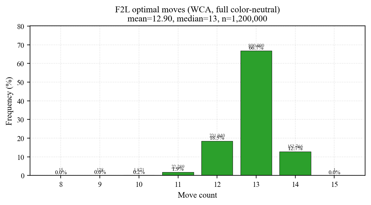
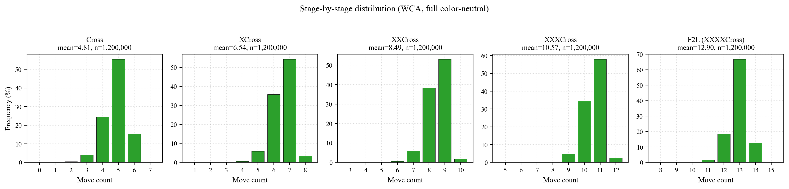
Three reads from the plots:
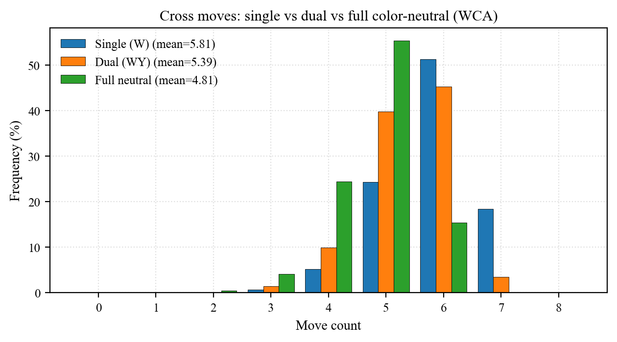
- Tight unimodal peaks: 45 ~ 67% of samples sit at the mode, std 0.6 ~ 0.8. The speedcuber's intuition "cross is usually 7 ~ 8" is empirically real — but std gives the mathematical lower bound, not a heuristic.
- ~2 moves per stage: 4.81 → 6.54 → 8.49 → 10.57 → 12.90. Each added pair costs slightly more than the last (+1.73, +1.96, +2.08, +2.33).
- Cross diameter ≤ 8 (single-color), F2L diameter = 15. The Cross-8 bound matches the long-known HTM result; F2L's longer tail reflects independent variance from 4 separate pairs.
Stage-to-stage mean increments (BGORWY)
| Transition | Mean Δ |
|---|---|
| XCross − Cross | +1.726 |
| XXCross − XCross | +1.957 |
| XXXCross − XXCross | +2.078 |
| F2L − XXXCross | +2.328 |
Color-neutrality marginal gain
Color neutrality (CN) means the solver can pick the most favourable bottom color at runtime. The std solver runs all 6 orientations per scramble; taking min over subsets quantifies the savings per added axis / colour.
The six orientations, geometrically
"Use a different bottom color" is equivalent to a cube-wide rotation applied to the scramble. The list in std_analyzer.cpp:
rots = { (identity), z², z', z, x', x }.These map to CSV columns _z0 / _z2 / _z3 / _z1 / _x3 / _x1, with bottom colors Y, W, O, R, G, B respectively. One scramble gives a 6-tuple of optimal step counts; any color-neutral subset (single / dual / quad / full) is just min over the relevant cells.
alg_rotation rewrites move indices according to these 8 basic rotations; the state object never changes:
y  : F→L→B→R→F    (顶面顺时针 90°)
y2 : F↔B,  L↔R
y' : F→R→B→L→F   (逆向)
z  : U→R→D→L→U
z2 : U↔D,  L↔R
z' : U→L→D→R→U
x  : U→F→D→B→U    (右侧顺时针 90°)
x' : U→B→D→F→U
Implementation: rotate the scramble, not the state
Two implementation paths: (1) rotate indices inside the state space; (2) rewrite the scramble itself. The latter is simpler and cache-friendly — std_analyzer picks it. alg_rotation(base_alg, rot) remaps every move index i (0..17) to its equivalent under the chosen rotation; the new alg is equivalent to base_alg but viewed from a different bottom color, and feeds straight into search. The whole analyzer runs on the "initial state + scramble sequence" abstraction with no physical-state-to-index converter anywhere.
From 6 views to 14 CN configurations
From the 6-tuple we derive 14 CN configurations: 6 singles / 3 duals (WY, BG, OR) / 3 quads (BGOR, ORWY, BGWY) / 1 hex (BGORWY full CN) / plus 1 baseline. Each configuration takes min over its colors, then we plot / aggregate the resulting distribution.
| Subset | Cardinality | Cross mean | Savings vs W |
|---|---|---|---|
| W (single) | 1 | 5.813 | 0 |
| WY (dual U/D) | 2 | 5.388 | −0.425 |
| BGOR / ORWY / BGWY (quad) | 4 | ~5.020 | −0.793 |
| BGORWY (full CN) | 6 | 4.811 | −1.002 |
Diminishing returns:
- 1 → 2 (W → WY): saves 0.425.
- 2 → 4 (WY → ORWY): another 0.368.
- 4 → 6 (ORWY → BGORWY): only 0.210 more.
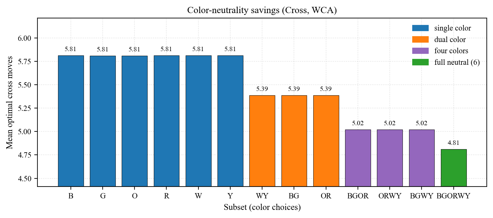
Takeaway: dual-axis CN (any opposite pair such as W-Y or B-G) is the best effort/return — about a third of the muscle-memory cost of full CN for ~53% of its mean savings. Going dual → full CN saves an extra ~0.58 moves on average but at the price of training all 6 orientations.
Empirical cubic symmetry
Cubic symmetry predicts the 6 single-color views (B / G / O / R / W / Y) to be statistically indistinguishable under a uniform scramble distribution. WCA scrambles are not strictly uniform (TNoodle plus history-weighted event mix), so any drift is informative. Cross stage 6 single-colour means:
| Bottom | Mean | std | p99 |
|---|---|---|---|
| B | 5.8135 | 0.8258 | 7 |
| G | 5.8115 | 0.8266 | 7 |
| O | 5.8111 | 0.8262 | 7 |
| R | 5.8125 | 0.8262 | 7 |
| W | 5.8129 | 0.8254 | 7 |
| Y | 5.8123 | 0.8261 | 7 |
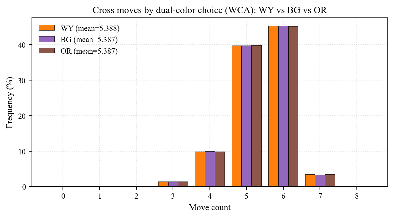
Single-colour mean spread 0.0025 moves. The 3 dual-color axes (W-Y, B-G, O-R) are also cube axes; selecting W-Y vs B-G vs O-R as the dual bottom should be statistically equivalent. On 1.2M WCA scrambles, std/Cross means (paper Table 10-1):
| Dual subset | Mean | Median | p99 | N |
|---|---|---|---|---|
| WY | 5.388 | 5 | 7 | 1,200,000 |
| BG | 5.388 | 5 | 7 | 1,200,000 |
| OR | 5.388 | 5 | 7 | 1,200,000 |
The three means agree within 0.001 moves — well inside 1.2M-sample noise. Cubic symmetry holds empirically, and the WCA scramble generator's distribution is uniform across the 6 bottom colors.
Hard-subset stress test
The second dataset (xcross_2_col_10f) is a deliberately collected WY-hard corpus: single-white XCross = 10 AND single-yellow XCross = 10. This pins a U/D-only solver at 10 moves on every one of 1.27M samples; BG / OR axes stay unconstrained, so full CN still has slack.
| Stage | WCA mean | Hard mean | Δ | WCA min | Hard min |
|---|---|---|---|---|---|
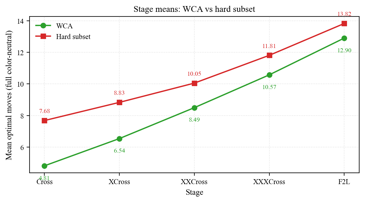
| Cross | 4.811 | 7.678 | +2.867 | 0 | 2 |
| XCross | 6.536 | 8.829 | +2.292 | 1 | 6 |
| XXCross | 8.493 | 10.049 | +1.555 | 3 | 8 |
| XXXCross | 10.572 | 11.808 | +1.236 | 5 | 9 |
| F2L | 12.900 | 13.824 | +0.924 | 8 | 10 |
An interesting decay: the filter is defined at XCross, but the largest Cross-stage shift is +2.87 — because forcing W-XCross = 10 nearly forces W-Cross to its max (single-W Cross = 8 in 1,271,514 / 1,271,727 ≈ 99.98% of hard samples). The shift decays monotonically through later stages, leaving only +0.92 at F2L. The hard-XCross tail does not propagate proportionally into the full F2L; this is the upper-bound flip-side of the admissible-lower-bound machinery.
A worked example
A single WCA historical scramble, id = 22001:
B2 U' L2 U F2 L2 D2 L2 U F2 L F2 L D U L' D2 F2' U2 B
std solver outputs across 6 bottom-color orientations, 5 stages each:
| Stage | Y | W | O | R | G | B | min |
|---|---|---|---|---|---|---|---|
| Cross | 6 | 6 | 6 | 5 | 7 | 5 | 5 |
| XCross | 7 | 7 | 8 | 7 | 9 | 7 | 7 |
| XXCross | 9 | 10 | 10 | 9 | 10 | 9 | 9 |
| XXXCross | 11 | 11 | 11 | 12 | 12 | 10 | 10 |
| F2L | 14 | 14 | 14 | 13 | 14 | 14 | 13 |
Full-CN stage trace: 5 / 7 / 9 / 10 / 13. From bottom-R the Cross is 5 moves; from bottom-G it is 7 — a 2-move spread that a CN solver would catch during inspection. F2L is 13 total, with Cross taking 5 ~ 8 of those moves. The F2L − Cross gap is 8, roughly matching the "3 F2L pairs + 1 XCross finisher" geometry.
Engineering + closing
Four design choices keep std fast and exact at once:
- O(1) move-table lookup: ~5 ns amortized per node.
- Admissible prune-table bound: guarantees optimality and pushes the IDA* start depth near the answer.
- Conjugation trick: 4 slots share a single precomputation.
- Cross-stage lower-bound propagation: F2L's iteration count is pinned by XXXCross's optimum — typically 1 ~ 3 rounds.
On 8 OpenMP threads, std_analyzer finishes 1000 WCA scrambles × 5 stages × 6 views in ~6 seconds. 1.2M samples take ~2 hours including Huge-table mmap warm-up. Table precomputation itself is ~1 hour, ~25 GB on disk (Huge alone 20 GB; if RAM is tight, keep it on SSD and mmap into the search loop). Huge tables are accessed via mmap on demand; the vast majority of queries hit the OS page cache and are not a bottleneck — that's what keeps the hot search loop near ~5 ns / node despite 10 GB tables.
- Correctness: 2.4M+ scrambles × 5 stages × 6 views ≈ 74M optimal searches finished without a single failure or precision anomaly — the implementation is empirically sound.
- Color-neutrality marginals: Cross saves 1.00 moves on average going from single to full CN. The first axis alone contributes 0.43; the remaining 4 axes combined only add 0.59 — textbook diminishing returns. Dual-axis CN is the best effort/return point.
- Cubic symmetry: on 1.2M samples the 3 dual-axis Cross means (W-Y / B-G / O-R) differ by < 0.001 moves — strictly within sampling noise. Cubic symmetry holds empirically, and the WCA scramble generator is symmetric on this sub-state space.
- Hard-subset behaviour: on 1.27M WY-hard samples, the mean shift vs WCA baseline narrows monotonically across stages (Cross +2.87 → F2L +0.92). All 5 stages still return optima; search time grows with difficulty but admissibility is unaffected.
The toolbox ports to other sub-goals. Replace the goal with "all 12 edges oriented" → EOCross solver, just needing a fresh mt_eo12 + matching prune table. Loosen the goal to "D-layer allowed a 90/180/270° offset" → pseudo variant, ~0.5 moves shorter on average. The Lehmer / move-table / prune-table / IDA* / conjugation / cross-stage-propagation scaffolding is shared across all four variants without modification.
Solving the 3×3 algorithmically is well-trodden — Kociemba's two-phase, Rokicki et al.'s 20-step diameter proof, Korf's pattern-database + IDA*. The std solver's distinguishing bits are two: hanging all 5 stages off one shared infrastructure, and pushing it through 1M+ real WCA scrambles to quantify per-stage distribution tails and color-neutrality marginals — quantities historically estimated on ~100k samples.
Future directions
Algorithm-side:
- Push more aggressive Pattern Databases: extend the current (Cross + 2 slots) Huge tables to (Cross + 3 slots), or compose them with cube-group automorphism equivalence classes to shrink storage while tightening h.
- Use GPU to accelerate the reverse-BFS prune-table build: Huge tables (~20 GB) take ~1 hour single-machine; GPU frontier-style BFS can shave an order of magnitude.
- Use neural networks for a non-admissible but on-average tighter heuristic: classical PDBs must satisfy h ≤ d* for optimality; an average-tighter learned h̃ would converge IDA* faster on most samples at the cost of giving up strict optimality (back to an "approximate + verify" metasolver). A favourable trade in applications that don't need absolute optima — e.g. training-system difficulty scoring.
Application-side:
- Wrap the solver as a real-time scramble analysis tool, embed it into trainer software, and use the output for objective scramble-difficulty / training-progress metrics.
- Build solve-visualisation and trainers on top of the 5-stage backbone: replay optimal solves stage-by-stage, compare a cuber's input to the optimum, deliver high-density Cross / F2L training feedback.